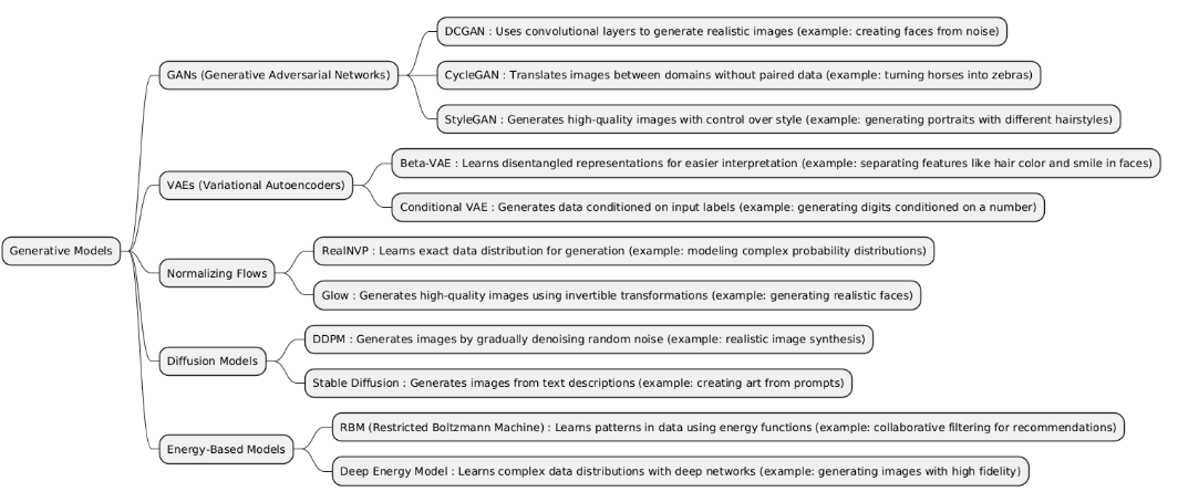
Generative Models are a class of machine learning models that learn to generate new data samples similar to the training data. They can create images, text, or other data types, and are widely used in applications like image synthesis, text generation, and data augmentation.
| Type | What it is | When it is used | When it is preferred over other types | When it is not recommended | Examples of projects that is better use it incide him |
|---|---|---|---|---|---|
| GANs | Generative Adversarial Networks (GANs) are deep generative models consisting of two networks — a generator that creates data and a discriminator that evaluates its authenticity — trained in an adversarial setup to produce realistic data samples. | Used for data generation, image synthesis, style transfer, super-resolution, and data augmentation. |
• Better than VAE for highly realistic and sharp images. • Faster than Diffusion Models for generating samples. • More suitable than Normalizing Flows when exact likelihood is not required but visual fidelity matters. • Better than Energy-Based Models for generating complex high-dimensional data with adversarial feedback. |
• When dataset is very small — GANs can be unstable. • When stable training or interpretability is critical. • When the task is representation learning rather than generation — VAE or flows may be better. |
• Image generation — generating realistic human faces (e.g., StyleGAN). • Image-to-image translation — converting sketches to photos. • Super-resolution — enhancing image resolution. • Data augmentation for training other models. • Artistic style transfer — applying painting styles to photos. |
| VAEs | Variational Autoencoders (VAEs) are generative models that learn a probabilistic latent representation of data. They encode inputs into a latent distribution and decode samples from it to reconstruct data. | Used for data generation, dimensionality reduction, anomaly detection, and representation learning. |
• Better than GANs when you need stable training and a well-defined latent space. • Better than Diffusion Models for faster sampling. • Better than Normalizing Flows when exact likelihood is less important and reconstruction matters. • Preferred over Energy-Based Models for explicit latent representation and reconstruction. |
• When highly realistic images are required — GANs or Diffusion Models may be better. • When exact likelihood estimation is needed — Normalizing Flows are preferable. • For tasks requiring sharp high-resolution outputs, VAEs tend to produce blurrier results. |
• Image generation — generating handwritten digits or faces. • Anomaly detection — detecting unusual medical images. • Representation learning — compressing data for downstream tasks. • Data augmentation — generating new synthetic samples for training classifiers. |
| Normalizing Flows | Normalizing Flows are generative models that transform a simple probability distribution (like Gaussian) into a complex data distribution using a sequence of invertible, differentiable transformations, allowing exact likelihood computation. | Used for density estimation, generative modeling, and likelihood-based tasks where exact probability calculation is important. |
• Better than GANs or Diffusion Models when exact likelihood evaluation is needed. • Better than VAEs if you require flexible distributions without approximate posterior sampling. • Preferred over Energy-Based Models for tractable training and exact likelihoods. |
• For high-resolution image generation where GANs or Diffusion Models produce sharper results. • When simplicity or training stability is desired — Normalizing Flows can be complex to implement. • For tasks focused on latent representations rather than exact density estimation — VAEs may be better. |
• Density estimation of molecular structures. • Anomaly detection in tabular or sensor data via likelihood evaluation. • Generating synthetic tabular data for simulations. • Probabilistic forecasting in finance or weather modeling. |
| Diffusion Models | Diffusion Models are generative models that iteratively transform noise into data through a reverse diffusion process, learning to generate complex data distributions step by step. | Used for high-quality image, audio, and video generation, especially where photo-realism and diversity are important. |
• Better than GANs when you need stable training and high-fidelity outputs. • Better than VAEs for sharp, detailed images. • Better than Normalizing Flows when exact likelihood is not required but sample quality matters. • Preferred over Energy-Based Models for faster and more reliable generation of realistic samples. |
• When fast sampling is required — Diffusion Models are slower than GANs or VAEs. • When computational resources are limited — training is heavy. • For tasks needing explicit latent representations — VAEs may be better. |
• Image generation — generating realistic human faces or artwork. • Text-to-image generation — creating images from captions. • Audio generation — producing realistic speech or music. • Video synthesis — generating short video clips from noise or conditional inputs. |
| EBMs | Energy-Based Models (EBMs) are generative models that assign an energy score to each configuration of variables, where lower energy means higher probability. They learn to model complex data distributions indirectly via this energy function. | Used for unsupervised learning, density estimation, and generative tasks, especially when modeling complex dependencies is needed. |
• Better than GANs or Diffusion Models when you want a flexible probabilistic model without requiring adversarial training. • Better than Normalizing Flows if exact invertibility is not needed but flexible modeling is. • Preferred over VAEs when you need to capture multi-modal distributions with complex correlations. |
• When sampling efficiency is critical — EBMs often require MCMC or iterative sampling. • For high-resolution image generation — GANs or Diffusion Models produce sharper outputs. • When interpretability or explicit latent space is needed — VAEs or Normalizing Flows are better. |
• Image generation — modeling complex image distributions. • Anomaly detection — detecting out-of-distribution samples by energy scores. • Molecular design — generating valid chemical structures. • Probabilistic modeling — learning distributions of physical systems or sensor data. |
import numpy as np
import matplotlib.pyplot as plt

# --- 1. Define latent vector (z) ---
latent_dim = 5
z = np.random.randn(latent_dim)  # random noise vector

# --- 2. Define a simple "style" mapping ---
def style_mapping(z):
    # Simulate the mapping network of StyleGAN
    return np.tanh(z * np.random.randn(*z.shape))

w = style_mapping(z)

# --- 3. Simple generator ---
def generator(w):
    # Simulate style-modulated generation
    img = np.zeros((16, 16))
    for i in range(16):
        for j in range(16):
            img[i, j] = np.sin(i * w[0] + j * w[1]) + np.cos(i * w[2] - j * w[3])
    img = (img - img.min()) / (img.max() - img.min())  # normalize 0-1
    return img

generated_image = generator(w)

# --- 4. Show image ---
plt.imshow(generated_image, cmap='gray')
plt.title("Generated Image (StyleGAN Concept)")
plt.axis('off')
plt.show()
import numpy as np
import matplotlib.pyplot as plt

# --- 1. Original image (simple 8x8 square) ---
true_image = np.zeros((8, 8))
true_image[2:6, 2:6] = 1.0  # white square

# --- 2. Forward diffusion (add noise step by step) ---
timesteps = 5
noisy_images = []
image = true_image.copy()
for t in range(timesteps):
    noise = np.random.randn(*image.shape) * (t + 1) / timesteps
    noisy_image = image + noise
    noisy_images.append(np.clip(noisy_image, 0, 1))

# --- 3. Reverse denoising process (simulate DDPM neural network) ---
denoised = noisy_images[-1].copy()
for t in reversed(range(timesteps)):
    # simple denoising step towards original image
    denoised = denoised - (denoised - true_image) * 0.2
    denoised = np.clip(denoised, 0, 1)

# --- 4. Show results ---
fig, axes = plt.subplots(1, 3, figsize=(9, 3))
axes[0].imshow(true_image, cmap='gray')
axes[0].set_title("Original Image")
axes[1].imshow(noisy_images[-1], cmap='gray')
axes[1].set_title("Noised Image")
axes[2].imshow(denoised, cmap='gray')
axes[2].set_title("Denoised (DDPM)")
plt.show()
import numpy as np
import matplotlib.pyplot as plt

# --- 1. Create a simple image (the "true" data") ---
true_image = np.zeros((28, 28))
true_image[10:18, 10:18] = 1.0  # simple white square

# --- 2. Forward diffusion process (add noise step by step) ---
timesteps = 10
noisy_images = []

image = true_image.copy()
for t in range(timesteps):
    noise = np.random.randn(*image.shape) * (t + 1) / timesteps
    noisy_image = image + noise
    noisy_images.append(np.clip(noisy_image, 0, 1))

# --- 3. Reverse denoising process (simulate the model learning to remove noise) ---
# In real Stable Diffusion, this is done by a neural network (U-Net + text encoder).
denoised = noisy_images[-1].copy()
for t in reversed(range(timesteps)):
    denoised = denoised - (denoised - true_image) * 0.2  # "denoise" toward target
    denoised = np.clip(denoised, 0, 1)

# --- 4. Show results ---
fig, axes = plt.subplots(1, 3, figsize=(9, 3))
axes[0].imshow(true_image, cmap='gray')
axes[0].set_title("Original Image")

axes[1].imshow(noisy_images[-1], cmap='gray')
axes[1].set_title("Noised (Forward Diffusion)")

axes[2].imshow(denoised, cmap='gray')
axes[2].set_title("Reconstructed (Reverse Diffusion)")

plt.show()